Linear Model (a single predictor)

# TODO: collect the installation of all necessary packages in one place at the beginning of the tutorial

#install.packages(c("ggplot2", "ggdist", "pwr"))

We start with the simplest possible linear model: (a) a continuous outcome variable is predicted by a single dichotomous predictor. This model actually rephrases a t-test as a linear model! Then we build up increasingly complex models: (b) a single continuous predictor and (c) multiple continuous predictors (i.e., multiple regression).

Data = Model + Error

The general equation for a linear model is:

\[y = b_0 + b_1*x_1 + b_2*x_2 + ... + e \tag{1}\]

where \(y\) is the continuous outcome variable, \(b_0\) is the intercept, \(x_1\) is the first predictor variable with its associated regression weight \(b_1\), etc. Finally, \(e\) is the error term which captures all variability in the outcome that is not explained by the predictor variables in the model. It is assumed that the error term is independently and identically distributed (iid) following a normal distribution with a mean of zero and a variance of \(\sigma^2\):

\[e \mathop{\sim}\limits^{\mathrm{iid}} N(mean=0, var=\sigma^2)\]

This assumption of the distribution of the errors is important for our simulations, as we will simulate the error according to that assumption. In an actual statistical analysis, the variance of the errors, \(\sigma^2\), is estimated from the data.

“i.i.d” means that the error of each observation is independent from all other observations. This assumption is violated, for example, when we look at romantic couples. If one partner is exceptionally disstressed, then the other partner presumably will also have higher stress levels. In this case, the errors of both partners are correlated, and not independent any more. (See the section on modelling multilevel data for a statistical way of handling such interdependences).

A concrete example

Let’s fill the abstract symbols of Equation 1 with some concrete content. Assume that we want to analyze the treatment effect of an intervention supposed to reduce depressive symptoms. In the study, a sample of participants with a diagnosed depression are randomized to either a control group or the treatment group.

We have the following two variables in our data set:

• BDI is the continuous outcome variable representing the severity of depressive symptoms after the treatment, assessed with the BDI-II inventory (higher values mean higher depression scores).
• treatment is our dichotomous predictor defining the random group assignment. We assign the following numbers: 0 = control group (e.g., an active control group), 1 = treatment group.

This is an opportunity to think about the actual scale of our variables. At the end, when we simulate data we need to insert concrete numbers into our equations:

• What BDI values would we expect on average in our sample (before treatment)?
• What variability would we expect in our sample?
• What average treatment effect would we expect?

All of these values are needed to be able to simulate data, and the chosen numbers imply a certain effect size.

Get some real BDI data as starting point

Note

The creators of this tutorial are no experts in clinical psychology; we opportunistically selected open data sets based on their availability. Usually, we would look for meta-analyses - ideally bias-corrected - for more comprehensive evidence.

The R package HSAUR contains open data on 100 depressive patients, where 50 received treatment-as-usual (TAU) and 50 received a new treatment (“Beat the blues”; BtheB). Data was collected in a pre-post-design with several follow-up measurements. For the moment, we focus on the pre-treatment baseline value (bdi.pre) and the first post-treatment value (bdi.2m). We will use that data set as a “pilot study” for our power analysis.

# the data can be found in the HSAUR package, must be installed first
#install.packages("HSAUR")

# load the data
data("BtheB", package = "HSAUR")

# get some information about the data set:
?HSAUR::BtheB

hist(BtheB$bdi.pre)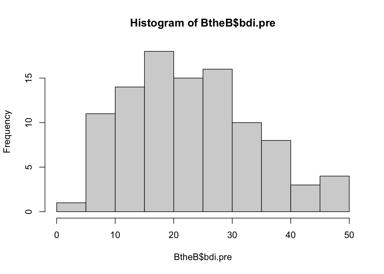

The standardized cutoffs for the BDI are:

• 0–13: minimal depression
• 14–19: mild depression
• 20–28: moderate depression
• 29–63: severe depression.

table(BtheB$bdi.pre >= 14) |> prop.table() |> round(2)

FALSE  TRUE 
  0.2   0.8 

Hence, 80% of participants had at least a “mild depression” before treatment according to these cutoffs.

Returning to our questions from above:

What BDI values would we expect on average in our sample (before treatment)?

# we take the pre-score here:
mean(BtheB$bdi.pre)

[1] 23.33

The average BDI score in that sample was 23, corresponding to a “moderate depression”.

• What variability would we expect in our sample?

var(BtheB$bdi.pre)

[1] 117.5163

• What average treatment effect would we expect?

# we take the 2 month follow-up measurement, 
# separately for the  "treatment as usual" and 
# the "Beat the blues" group:
mean(BtheB$bdi.2m[BtheB$treatment == "TAU"], na.rm=TRUE)

[1] 19.46667

mean(BtheB$bdi.2m[BtheB$treatment == "BtheB"])

[1] 14.71154

Hence, the two treatments reduced BDI scores from an average of 23 to 19 (TAU) and 15 (BtheB). Based on that data set, we can conclude that a typical treatment effect is somewhere between a 4 and a 8-point reduction of BDI scores.¹

For our purpose, we compute the average treatment effect combined for both treatments. The average post-treatment score is:

mean(BtheB$bdi.2m, na.rm=TRUE)

[1] 16.91753

So, the average reduction across both treatments is \(17-23=6\).

Enter specific values for the model parameters

Let’s rewrite the abstract equation with the specific variable names. We first write the equation for the systematic part (without the error term). This also represents the predicted value:

\[\widehat{\text{BDI}} = b_0 + b_1*\text{treatment} \tag{2}\]

We use the notation \(\widehat{\text{BDI}}\) (with a hat) to denote the predicted BDI score.

The predicted score for the control group then simply is the intercept of the model, as the second term is erased by entering the value “0” for the control group:

\[\widehat{\text{BDI}} = b_0 + b_1*0 = b_0\]

The predicted score for the treatment group is the value for the control group plus the regression weight:

\[\widehat{\text{BDI}} = b_0 + b_1*1\] Hence, the regression weight (aka. “slope parameter”) \(b_1\) estimates the mean difference between both groups, which is the treatment effect.

With our knowledge from the open BDI data, we insert plausible values for the intercept \(b_0\) and the treatment effect \(b_1\). We expect a reduction of the depression score, so the treatment effect is assumed to be negative. We take the combined treatment effect of the two pilot treatments. And as power analysis is not rocket science, we generously round the values:

\[\widehat{\text{BDI}} = 23 - 6*treatment\]

Hence, the predicted value is \(23 - 6*0 = 23\) for the control group, and \(23 - 6*1 = 17\) for the treatment group.

With the current model, all persons in the control group have the same predicted value (23), as do all persons in the treatment group (17).

As a final step, we add the random noise to the model, based on the variance in the pilot data:

\[\text{BDI} = 23 - 6*treatment + e; e \sim N(0, var=117) \]

That’s our final equation with assumed population parameters! With that equation, we assume a certain state of reality and can sample “virtual participants”.

What is the effect size in the model?

The raw effect size is simply the treatment effect on the original BDI scale (i.e., the group difference in the outcome variable). In our case we assume that the treatment lowers the BDI score by 6 points, on average. The standardized effect size relates the raw effect size to the variability. In the two-group example, this can be expressed as Cohen’s d, which is the mean difference divided by the standard deviation (SD):

\[d = \frac{M_{treat} - M_{control}}{SD} = \frac{17 - 23}{\sqrt{117}} = -0.55\]

Note

If you look up the formula of Cohen’s d, it typically uses the pooled SD from both groups. As we assumed that both groups have the same SD, we simply took that value.

Let’s simulate!

Once we committed to an equation with concrete parameter values, we can simulate data for a sample of, say, \(n=100\) participants. Simply write down the equation and add random normal noise with the rnorm function. Note that the rnorm function takes the standard deviation (not the variance). Finally, set a seed so that the generated random numbers are reproducible:

set.seed(0xBEEF)

# define all simulation parameters and predictor variables:
n <- 50
treatment <- c(rep(0, n/2), rep(1, n/2)) # first 50 control, then 50 treatment

# Write down the equation
BDI <- 23 - 6*treatment + rnorm(n, mean=0, sd=sqrt(117))

# combine all variables in one data frame
df <- data.frame(treatment, BDI)

head(df)

  treatment      BDI
1         0 29.37241
2         0 25.49819
3         0 18.80709
4         0 14.52574
5         0 11.79615
6         0 10.98850

tail(df)

   treatment       BDI
45         1 25.871732
46         1 27.744107
47         1 20.749970
48         1 40.275788
49         1  2.981421
50         1  8.151660

Let’s plot the simulated data with raincloud plots (see here for a tutorial):

library(ggplot2)
ggplot(df, aes(x=as.factor(treatment), y=BDI)) + 
  ggdist::stat_halfeye(adjust = .5, width = .3, .width = 0, justification = -.3, point_colour = NA) + 
  geom_boxplot(width = .1, outlier.shape = NA) +
  gghalves::geom_half_point(side = "l", range_scale = .4, alpha = .5)

Let’s assume that we collected and analyzed this sample - what would have been the results?

summary(lm(BDI ~ treatment, data=df))

Call:
lm(formula = BDI ~ treatment, data = df)

Residuals:
     Min       1Q   Median       3Q      Max 
-24.8539  -7.9693   0.5002   7.7587  23.7909 

Coefficients:
            Estimate Std. Error t value Pr(>|t|)    
(Intercept)   24.975      2.318  10.776 2.07e-14 ***
treatment     -7.787      3.278  -2.376   0.0216 *  
---
Signif. codes:  0 '***' 0.001 '**' 0.01 '*' 0.05 '.' 0.1 ' ' 1

Residual standard error: 11.59 on 48 degrees of freedom
Multiple R-squared:  0.1052,    Adjusted R-squared:  0.08656 
F-statistic: 5.643 on 1 and 48 DF,  p-value: 0.02156

Here, and in the entire tutorial, we assume an \(\alpha\)-level of .005 (Benjamin et al., 2018). As you can see, in this specific sample the treatment effect is not significant at p > .02. But maybe in another sample of the same size?

Doing the power analysis

Now we need to repeatedly draw many samples and see how many of the analyses would have detected the existing effect. To do this, we put the code from above into a loop and repeatedly do the procedure.

set.seed(0xBEEF)

# define all predictor and simulation variables.
# (we do this outside the loop as it stays constant)
iterations <- 1000
n <- 100
treatment <- c(rep(0, n/2), rep(1, n/2))

# vector that collects the p-values from all 1000 virtual samples
# (prepare an empty NA vector with 1000 slots)
p_values <- rep(NA, iterations)

# now repeatedly draw samples, analyze, and the p-value of the 
# focal regression weight (i.e., the slope parameter)
for (i in 1:iterations) {
  BDI <- 23 - 6*treatment + rnorm(n, mean=0, sd=sqrt(117))
  res <- lm(BDI ~ treatment)
  p_values[i] <- summary(res)$coefficients["treatment", "Pr(>|t|)"]
}

How many of our 1000 virtual samples would have found the effect?

table(p_values < .005)

FALSE  TRUE 
  535   465 

Only 46% of samples with the same size of \(n=100\) result in a significant p-value.

46% - that is our power for \(\alpha = .005\), Cohen’s \(d=.55\), and \(n=100\).

Sample size planning: Find the necessary sample size

Now we know that a sample size of 100 does not lead to a sufficient power. But what sample size would we need to achieve a power of at least 80%? In the simulation approach you need to test different \(n\)s until you find the necessary sample size. We do this by wrapping the simulation code into another loop that continuously increases the n. We then store the computed power for each n.

set.seed(0xBEEF)

# define all predictor and simulation variables.
iterations <- 1000
ns <- seq(100, 300, by=20) # test ns between 100 and 400

result <- data.frame()

for (n in ns) {  # outer loop
  treatment <- c(rep(0, n/2), rep(1, n/2))
  p_values <- rep(NA, iterations)

  # now repeatedly draw samples, analyze, and save p-value
  for (i in 1:iterations) {  # inner loop
    BDI <- 23 - 6*treatment + rnorm(n, mean=0, sd=sqrt(117))
    res <- lm(BDI ~ treatment)
    p_values[i] <- summary(res)$coefficients["treatment", "Pr(>|t|)"]
  } 
  
  result <- rbind(result, data.frame(
    n = n,
    power = sum(p_values < .005)/iterations)
  )
  
  # show the result after each run (not shown here in the tutorial)
  print(result)
}

Let’s plot there result:

ggplot(result, aes(x=n, y=power)) + geom_point() + geom_line()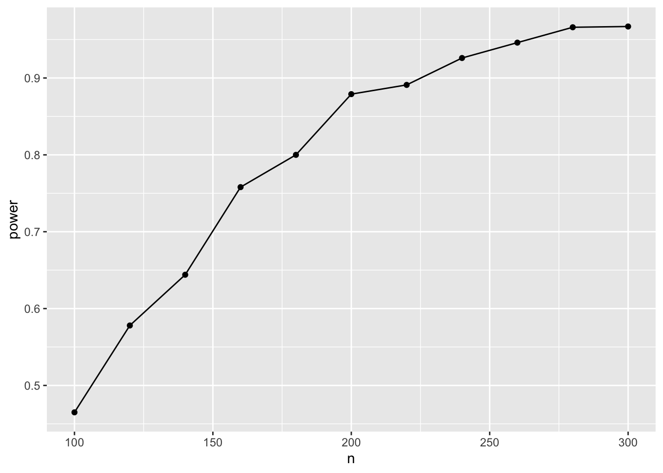

Hence, with n=180 (90 in each group), we have a 80% chance to detect the effect.

🥳 Congratulations! You did your first power analysis by simulation. 🎉

For these simple models, we can also compute analytic solutions. Let’s verify our results with the pwr package:

library(pwr)
pwr.t.test(d = 0.55, sig.level = 0.005, power = .80)

     Two-sample t test power calculation 

              n = 90.00212
              d = 0.55
      sig.level = 0.005
          power = 0.8
    alternative = two.sided

NOTE: n is number in *each* group

Exactly the same result - phew 😅

Sensitivity analyses

When we entered the specific numbers into our equations, we used point estimates from a relatively small pilot sample. As there is considerable uncertainty around these estimates, the true population value could be much smaller or larger. Therefore, we will explore two other ways to set the effect size: safeguard power analysis and the smallest effect size of interest (SESOI).

Safeguard power analysis

As sensitivity analysis, we will apply a safeguard power analysis, that aims for the lower end of a two-sided 60% CI around the parameter of the focal treatment effect (the intercept is irrelevant). (Of course you can use any other value than 60%, but this is the value (tentatively) mentioned by the inventors of the safeguard power analysis.)

Note

If you assume publication bias, another heuristic for aiming at a more realistic population effect size is the “divide-by-2” heuristic. (TODO: Link to presentation)

We can use the t.test function to compute a CI around that value:

t.test(BtheB$bdi.2m, BtheB$bdi.pre, na.rm=TRUE, conf.level = 0.60)

    Welch Two Sample t-test

data:  BtheB$bdi.2m and BtheB$bdi.pre
t = -4.1613, df = 194.87, p-value = 4.745e-05
alternative hypothesis: true difference in means is not equal to 0
60 percent confidence interval:
 -7.712244 -5.112704
sample estimates:
mean of x mean of y 
 16.91753  23.33000 

MOTE Online Calculator

You can also use the MOTE online calculator by Erin Buchanan et al. to compute effect sizes and confidence intervals around them: https://doomlab.shinyapps.io/mote/

This takes either raw statistics (means, SDs) or test statistics as input.

As the assumed effect is negative, we aim for the upper, i.e., the more conservative limit, which is considerably smaller, at -5.1.

Tip: Computing CIs around standardized effect sizes

When you use a standardized mean difference that has been reported in a paper, you can use a function from the MBESS package to compute the CI:

library(MBESS)

# smd = standardized mean difference = Cohen's d
ci.smd(smd=0.55, n.1=50, n.2=50, conf.level=0.60)

Now we can rerun the power simulation with this more conservative value (the only change to the code above is that we changed the treatment effect from -6 to -5.1).

Show the code

set.seed(0xBEEF)

# define all predictor and simulation variables.
iterations <- 1000
ns <- seq(100, 300, by=20)

result <- data.frame()

for (n in ns) {
  treatment <- c(rep(0, n/2), rep(1, n/2))
  p_values <- rep(NA, iterations)

  # now repeatedly draw samples, analyze, and save p-value of 
  for (i in 1:iterations) {
    BDI <- 23 - 5.1*treatment + rnorm(n, mean=0, sd=sqrt(117))
    res <- lm(BDI ~ treatment)
    p_values[i] <- summary(res)$coefficients["treatment", "Pr(>|t|)"]
  } 
  
  result <- rbind(result, data.frame(
    n = n,
    power = sum(p_values < .005)/iterations)
  )
  
  # show the result after each run
  print(result)
}

     n power
1  100 0.314
2  120 0.408
3  140 0.473
4  160 0.570
5  180 0.618
6  200 0.717
7  220 0.735
8  240 0.795
9  260 0.823
10 280 0.878
11 300 0.887

With that more conservative effect size assumption, we would need around 240 participants, i.e. 120 per group.

Smallest effect size of interest (SESOI)

Many methodologists argue that we should not power for the expected effects size, but rather for the smallest effect size of interest. In this case, a non-significant result can be interpreted as “We accept the \(H_0\), and even if a real effect existed, it most likely is too small to be relevant”.

What change of BDI scores is perceived as “clinically important”? The hard part is to find a convincing theoretical or empirical argument for the chosen SESOI. In the case of the BDI, luckily someone else did that work.

The NICE guidance suggest that a change of >=3 BDI-II points is clinically important.

However, as you can expect, things are more complicated. Button et al. (2015) analyzed data sets where patients have been asked, after a treatment, whether they felt “better”, “the same” or “worse”. With these subjective ratings, they could relate changes in BDI-II scores to perceived improvements. Hence, even when depressive symptoms where measureably reduced in the BDI, patients still might answer “feels the same”, which indicates that the reduction did not surpass a threshold of subjective relevant improvement. For example, the minimal clinical importance depends on the baseline severity: For patients to feel notably better, they need more reduction of BDI-II scores if they start from a higher level of depressive symptoms. Following from this analysis, typical SESOIs are higher than the NICE guidelines, more in the range of -6 BDI points.

Let’s use the NICE recommendation of -3 BDI points as a lower threshold for our power analysis (anything larger than that will be covered anyway).

Show the code

set.seed(0xBEEF)

# define all predictor and simulation variables.
iterations <- 1000
ns <- seq(600, 800, by=20)

result <- data.frame()

for (n in ns) {
  treatment <- c(rep(0, n/2), rep(1, n/2))
  p_values <- rep(NA, iterations)

  # now repeatedly draw samples, analyze, and save p-value of 
  for (i in 1:iterations) {
    BDI <- 23 - 3*treatment + rnorm(n, mean=0, sd=sqrt(117))
    res <- lm(BDI ~ treatment)
    p_values[i] <- summary(res)$coefficients["treatment", "Pr(>|t|)"]
  } 
  
  result <- rbind(result, data.frame(
    n = n,
    power = sum(p_values < .005)/iterations)
  )
}

     n power
1  600 0.728
2  620 0.738
3  640 0.756
4  660 0.781
5  680 0.791
6  700 0.791
7  720 0.827
8  740 0.820
9  760 0.852
10 780 0.866
11 800 0.871

Hence, we need around 700 participants to reliably detect this smallest effect size of interest.

Did you spot the strange pattern in the result? At n=720, the power is 83%, but only 82% with n=740? This is not possible and suggests that this is simply Monte Carlo sampling error - 1000 iterations is not enough to get precise estimates. When we increase iterations to 10,000, it takes much longer, but gives more precise results:

Show the code

set.seed(0xBEEF)

# define all predictor and simulation variables.
iterations <- 10000

# To speed up computations, we limited the range of ns to the relevant region
ns <- seq(640, 740, by=20)

result <- data.frame()

for (n in ns) {
  treatment <- c(rep(0, n/2), rep(1, n/2))
  p_values <- rep(NA, iterations)

  # now repeatedly draw samples, analyze, and save p-value of 
  for (i in 1:iterations) {
    BDI <- 23 - 3*treatment + rnorm(n, mean=0, sd=sqrt(117))
    res <- lm(BDI ~ treatment)
    p_values[i] <- summary(res)$coefficients["treatment", "Pr(>|t|)"]
  } 
  
  result <- rbind(result, data.frame(
    n = n,
    power = sum(p_values < .005)/iterations)
  )
  
  # show the result after each run
  print(result)
}

     n  power
1  600 0.7244
2  620 0.7353
3  640 0.7528
4  660 0.7721
5  680 0.7889
6  700 0.8001
7  720 0.8150
8  740 0.8328
9  760 0.8374
10 780 0.8573
11 800 0.8682

Now the power increases monotonically with sample size, as expected.

Recap: What did we do?

These are the steps we did in the tutorial:

1. Define the statistical model that you will use to analyze your data (in our case: a linear regression). This sometimes is called the data generating mechanism or the data generating model.
2. Find empirical information about the parameters in the model. These are typically mean values, variances, group differences, regression coefficients, or correlations (in our case: a mean value (before treatment), a group difference, and an error variance). These numbers define your assumed state of the population.
3. Program your equation, which consists of a systematic (i.e., deterministic) part and (one or more) random error terms.
4. Do the simulation:
   1. Repeatedly sample data from your equation (only the random error changes in each run, the deterministic part stays the same)
   2. Compute the index of interest (typically: the p-value of a focal effect)
   3. Count how many samples would have detected the effect
   4. Tune your simulation parameters until the desired level of power is achieved

Concerning step 4d, the typical scenario is that you increase sample size until your desired level of power is achieved. But you could imagine other ways to increase power, e.g.:

• increase the reliability of a measurement instrument (which will be reflected in a larger effect size) until desired power is achieved. (This could relate to a trade-off: Do you invest more effort and time in better measurement, or do you keep an unreliable measure and collect more participants?)
• Compare a within- and a between-design in simulations
• … TODO

Bonus 1: Beyond power: General design analysis

TBD:

• Compute another quantity of interest (e.g., the width of a CI), and optimize the sample size for that.

Bonus 2: Optimizing your code for speed

TBD

system.time({
  
# vectors that collect the results
p_values <- rep(NA, iterations)

# now repeatedly draw samples, analyze, and save p-value of 
for (i in 1:iterations) {
  print(i) # show how long we have to wait ...
  BDI <- 23 - 6*treatment + rnorm(n, mean=0, sd=sqrt(117))
  res <- lm(BDI ~ treatment)
  p_values[i] <- summary(res)$coefficients["treatment", "Pr(>|t|)"]
}
  
})

Generally, you can start with few iterations for a fast exploration of the parameter space. When you found the relevant range (e.g., the necessary sample size to achieve a power between 70% and 90 %), you can restrict the parameter space to that range and increase the number of iterations to get more precise results.

Bonus 3: The quick solution: sampling from pilot samples

If your pilot study has exactly the same data structure as the study you are planning for you can take the resulting lm object and directly sample from that.

With that procedure, however, you assume that the pilot study perfectly hit the true effect size (and all other parameters of the model)

References

Button, K. S., Kounali, D., Thomas, L., Wiles, N. J., Peters, T. J., Welton, N. J., Ades, A. E., & Lewis, G. (2015). Minimal clinically important difference on the Beck Depression Inventory—II according to the patient’s perspective. Psychological Medicine, 45(15), 3269–3279. https://doi.org/10.1017/S0033291715001270

Footnotes

1. By comparing only the post-treatment scores we used an unbiased causal model for the treatment effect. Later we will increase the precision of the estimate by including the baseline score into the model.