Bonus: How many Monte-Carlo iterations are necessary?

Using the optimized code, we can easily explore how many Monte-Carlo iterations are necessary to get stable computational results: Simply re-run the same simulation with the same sample size!

Let’s start with 1000 iterations (at n = 100, and 10 repetitions of the same power analysis):

set.seed(0xBEEF)
iterations <- 1000

# CHANGE: do the same sample size repeatedly, and see how much different runs deviate.
ns <- rep(100, 10)

result <- data.frame()

for (n in ns) {
  
  x <- cbind(
    rep(1, n),
    c(rep(0, n/2), rep(1, n/2))
  )
  
  p_values <- rep(NA, iterations)
  
  for (i in 1:iterations) {
    y <- 23 - 3*x[, 2] + rnorm(n, mean=0, sd=sqrt(117))
    
    mdl <- RcppArmadillo::fastLmPure(x, y)
    pval <- 2*pt(abs(mdl$coefficients/mdl$stderr), mdl$df.residual, lower.tail=FALSE)
    
    p_values[i] <- pval[2]
  }
  
  result <- rbind(result, data.frame(n = n, power = sum(p_values < .005)/iterations))
}

result

     n power
1  100 0.065
2  100 0.070
3  100 0.068
4  100 0.066
5  100 0.067
6  100 0.073
7  100 0.071
8  100 0.070
9  100 0.071
10 100 0.063

As you can see, the power estimates show some variance, ranging from 0.063 to 0.073. This can be formalized as the Monte-Carlo error (MCE), which is define as “the standard deviation of the Monte Carlo estimator, taken across hypothetical repetitions of the simulation” (Koehler et al., 2009). With 1000 iterations (and 10 repetitions), this is:

sd(result$power) |> round(4)

[1] 0.0031

We only computed 10 repetitions of our power estimate, hence the MCE estimate is quite unstable. In the next computation, we will compute 100 repetitions of each power estimate.

How much do we have to increase the iterations to achieve a MCE smaller than, say, 0.005 (i.e, an SD of +/- 0.5% of the power estimate)?

Let’s loop through increasing iterations (this takes a few minutes):

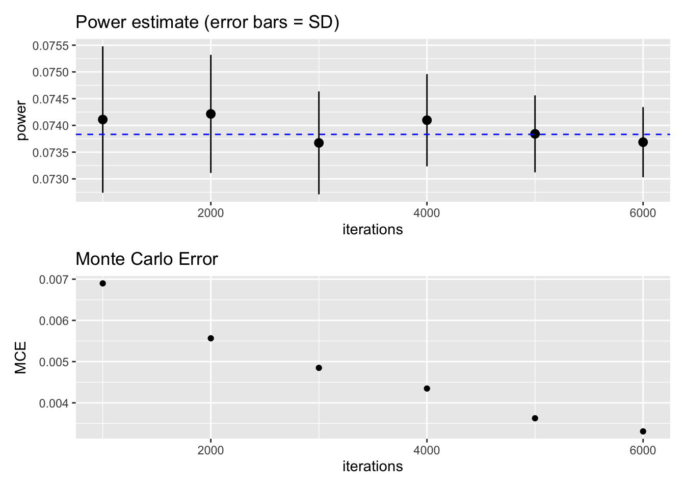
library(RcppArmadillo)
iterations <- seq(1000, 6000, by=1000)

# let's have 100 iterations to get sufficiently stable MCE estimates
ns <- rep(100, 100)
result <- data.frame()

for (it in iterations) {

  # print(it)  uncomment for showing the progress

  for (n in ns) {
    
    x <- cbind(
      rep(1, n),
      c(rep(0, n/2), rep(1, n/2))
    )
    
    p_values <- rep(NA, it)
    
    for (i in 1:it) {
      y <- 23 - 3*x[, 2] + rnorm(n, mean=0, sd=sqrt(117))
      
      mdl <- RcppArmadillo::fastLmPure(x, y)
      pval <- 2*pt(abs(mdl$coefficients/mdl$stderr), mdl$df.residual, lower.tail=FALSE)
      
      p_values[i] <- pval[2]
    }
    
    result <- rbind(result, data.frame(iterations = it, n = n, power = sum(p_values < .005)/it))
  }
}

library(ggplot2)
library(patchwork)
library(pwr)

# We can compute the exact power with the analytical solution:
exact_power <- pwr.t.test(d = 3 / sqrt(117), sig.level = 0.005, n = 50)

p1 <- ggplot(result, aes(x=iterations, y=power)) + stat_summary(fun.data=mean_cl_normal) + ggtitle("Power estimate (error bars = SD)") + geom_hline(yintercept = exact_power$power, colour = "blue", linetype = "dashed")

p2 <- ggplot(result, aes(x=iterations, y=power)) + stat_summary(fun="sd", geom="point") + ylab("MCE") + ggtitle("Monte Carlo Error")

p1/p2

As you can see, the MCE gets smaller with increasing iterations. The desired precision of MCE <= .005 can be achieved at around 3000 iterations (the dashed blue line is the exact power estimate from the analytical solution). While precision increases quickly by going from 1000 to 2000 iterations, further improvements are costly in terms of computation time. In sum, 3000 iterations seems to be a good compromise for this specific power simulation.

Note

This choice of 3000 iterations does not necessarily generalize to other power simulations with other statistical models. But in my experience, 2000 iterations typically is a good (enough) choice. I often start with 500 iterations when exploring the parameter space (i.e., looking roughly for the range of reasonable sample sizes), and then “zoom” into this range with 2000 iterations.

In the lower plot, you can also see that the MCE estimate itself is a bit wiggly - we would expect a smooth curve. It suffers from meta-MCE! We could increase the precision of the MCE estimate by increasing the number of repetitions (currently at 100).